How Is NGS Analysis Performed? Step-by-Step NGS Workflow -

Next-generation sequencing (NGS) has transformed genomics by making it possible to analyze millions to billions of DNA or RNA sequences in a single experiment. However, NGS analysis is much more than simply sequencing a biological sample and looking for variants.

A complete NGS workflow begins long before the sequencing instrument generates reads. Sample quality, library preparation, sequencing parameters, quality control, read preprocessing, alignment or transcript quantification, variant calling, annotation, biological interpretation, and reporting all influence the reliability of the final result.

Depending on the application, an NGS workflow may be used for:

- Whole Genome Sequencing (WGS)
- Whole Exome Sequencing (WES)
- Targeted gene panels
- Germline variant analysis
- Somatic variant analysis
- Hereditary cancer analysis
- Carrier screening
- RNA sequencing (RNA-Seq)
- Transcriptome analysis
- Copy number variation analysis CNV
- Structural variant analysis (SV)
- Mitochondrial DNA analysis mtDNA
- Microbial sequencing
- Metagenomics
- Pharmacogenomics
- Research and clinical genomics

Although the exact pipeline depends on the sequencing technology and biological question, the overall process can be represented as:

Sample → Nucleic Acid Extraction → QC → Library Preparation → Sequencing → Raw Data → Read QC → Preprocessing → Alignment/Quantification → Variant or Expression Analysis → Annotation → Interpretation → Reporting

This article explains each stage in detail and describes what happens to the data from the biological sample all the way to the final analytical result.

What Is NGS Analysis?

Next-generation sequencing refers to high-throughput sequencing technologies capable of generating very large numbers of sequence reads in parallel.

Unlike traditional Sanger sequencing, which generally analyzes a relatively small number of DNA fragments at a time, NGS platforms generate millions or billions of reads during a sequencing run.

The fundamental objective of NGS analysis is to convert these raw sequencing reads into biologically meaningful information.

For example, in a germline WES experiment, the analytical process may ultimately answer questions such as:

Which genetic variants are present?
Which variants are rare in the population?
Which genes are affected?
Which variants alter protein sequence?
Which variants have previously been associated with disease?
Which variants are potentially pathogenic?
Which variants should be prioritized for further investigation?

In RNA-Seq, the questions are different:

Which genes are expressed?
How strongly are they expressed?
Which transcripts are present?
Which genes are differentially expressed between conditions?
Are there alternative splicing events?
Are fusion transcripts present?

Therefore, there is no single universal NGS analysis pipeline.

The pipeline must be designed according to the:

Sample type
Sequencing technology
Experimental design
Sequencing strategy
Biological question
Desired variant types
Clinical or research objective

The Complete NGS Workflow at a Glance

A typical DNA-based NGS workflow can be divided into several major stages.

Wet-lab workflow

Sample collection
DNA/RNA extraction
Nucleic acid quality control
Library preparation
Library QC
Library pooling
Sequencing

Bioinformatics workflow

Raw data generation
Raw read quality control
Adapter and quality trimming
Reference genome preparation
Read alignment
Alignment QC
Duplicate marking
Base quality recalibration or platform-specific preprocessing
Variant calling
Variant quality filtering
Variant annotation
Variant prioritization
Variant interpretation
Clinical/biological reporting

The exact workflow varies according to whether the analysis is WGS, WES, targeted sequencing, RNA-Seq, or another application.

Step 1: Define the Biological and Analytical Objective

Before sequencing begins, the most important question is: What biological question are we trying to answer?

This determines almost every downstream decision.

For example:

Whole Genome Sequencing

WGS analyzes genomic regions across essentially the entire genome.

It can be used for:

SNVs
Small insertions and deletions
CNVs
Structural variants
Non-coding variants
Mitochondrial variants
Population genomics

Whole Exome Sequencing

WES focuses primarily on protein-coding regions of the genome.

It is commonly used for:

Rare disease research
Mendelian disorders
Germline variant discovery
Gene discovery
Clinical genetics

Targeted Gene Panels

Targeted sequencing focuses on a predefined set of genes or genomic regions.

Advantages include:

High sequencing depth
Lower sequencing cost
Efficient analysis
Easier variant interpretation

RNA-Seq

RNA sequencing is designed to study the transcriptome rather than genomic DNA.

It can be used to investigate:

Gene expression
Differential expression
Alternative splicing
Transcript abundance
Gene fusions
Novel transcripts

Therefore, the first stage of a successful NGS project is not sequencing itself. It is experimental and analytical design.

Step 2: Sample Collection and Nucleic Acid Extraction

The NGS workflow starts with biological material.

Depending on the application, samples may include:

Whole blood
Saliva
Buccal cells
Tissue
Tumor tissue
FFPE tissue
Bone marrow
Cell cultures
Fresh or frozen tissue
Plasma
Other biological fluids

The extraction method depends on the type of nucleic acid being analyzed.

For DNA sequencing, genomic DNA is extracted.

For RNA sequencing, total RNA or another RNA fraction may be extracted.

The quality of the starting material can have a major impact on downstream sequencing.

Illumina describes nucleic acid isolation as the first stage of the overall NGS workflow, followed by quality control, library preparation, sequencing, and analysis.

Step 3: Nucleic Acid Quality Control

Before library preparation, DNA or RNA must be evaluated.

Several parameters may be examined.

Concentration

The amount of nucleic acid must be sufficient for the selected library preparation protocol.

Quantification can be performed using methods such as:

Fluorometric assays
Spectrophotometry
Other platform-specific quantification methods

Fluorometric methods are generally more specific for nucleic acid quantification, while spectrophotometry can provide information about purity. Illumina specifically recommends fluorometric methods for quantitation and UV spectrophotometry for purity assessment.

Purity

Potential contaminants can interfere with downstream enzymatic reactions.

Common purity measurements include:

A260/A280
A260/A230

Unexpected ratios may indicate contamination by:

Proteins
Phenol
Salts
Carbohydrates
Other extraction reagents

DNA Integrity

DNA fragmentation can influence library preparation and sequencing performance.

This is particularly important for:

FFPE samples
Degraded clinical samples
Archived material

High-quality intact DNA generally provides greater flexibility for downstream applications.

RNA Quality

RNA analysis requires additional quality assessment.

RNA degradation can significantly affect RNA-Seq results.

Depending on the workflow, metrics such as:

RNA Integrity Number (RIN)
DV200
RNA concentration

may be evaluated.

Poor RNA integrity can alter transcript representation and introduce bias into expression analysis.

Step 4: Library Preparation

Sequencing instruments generally do not directly sequence the original genomic DNA molecule in its raw form.

Instead, the DNA or RNA-derived material is converted into a sequencing library.

Library preparation is therefore one of the most important stages of the NGS workflow.

Illumina describes library preparation as the process of converting genomic DNA or cDNA into a library of fragments suitable for sequencing.

A typical DNA library preparation workflow can include:

DNA fragmentation
End repair
A-tailing, depending on protocol
Adapter ligation
Index/barcode addition
PCR amplification, depending on protocol
Library purification
Library QC

What Are Sequencing Adapters?

Adapters are short DNA sequences attached to library fragments.

They allow sequencing instruments to:

Recognize library molecules
Attach molecules to the sequencing surface
Initiate sequencing
Identify individual libraries in multiplexed experiments

Adapters can also contain index sequences.

What Is Multiplexing?

Multiplexing allows multiple samples to be sequenced in the same sequencing run.

Each library receives a unique index or barcode.

During bioinformatics processing, reads can then be assigned back to their corresponding samples.

This process is called:

Demultiplexing

A simplified representation is:

Sample A → Index A ┐
Sample B → Index B ├──→ Sequencing Run → Demultiplexing → Individual FASTQ files
Sample C → Index C ┘

Multiplexing can significantly increase sequencing efficiency because multiple samples share the same sequencing run.

However, incorrect indexing, index hopping, contamination, or sample mix-ups can compromise downstream analysis.

Step 5: Library Quality Control

After library preparation, the libraries themselves should be evaluated.

Typical parameters include:

Library concentration
Fragment size distribution
Adapter contamination
Library integrity

The expected fragment size depends on the library preparation protocol and sequencing strategy.

The library is then typically normalized and pooled before sequencing.

Step 6: Sequencing

The prepared libraries are loaded onto a sequencing instrument.

Different sequencing platforms use different technologies.

For example, Illumina sequencing systems use sequencing-by-synthesis chemistry, in which incorporated bases are detected during synthesis of the complementary DNA strand.

Sequencing generates millions or billions of individual reads.

Important sequencing parameters include:

Read length

The number of bases sequenced per read.

Examples include:

75 bp
100 bp
150 bp
Longer reads depending on platform

Sequencing depth

The number of times a genomic position is represented by sequencing reads.

For example, approximately 30× WGS means that a genomic position is represented by an average of about 30 reads.

Coverage

Coverage describes how much of the target region is sufficiently represented by sequencing data.

Depth and coverage are related but are not identical.

A sample can have high average depth but poor coverage of particular genomic regions.

Single-End vs Paired-End Sequencing

Two common sequencing strategies are:

Single-End

The fragment is sequenced from one end.

Fragment
|------------------------------|
→→→→→→→→→→→→→→

Paired-End

The fragment is sequenced from both ends.

Fragment
|------------------------------|
→→→→→→→→→→→→→→
←←←←←←←←←←←←←←

Paired-end sequencing can provide additional information about:

Read alignment
Insert size
Repetitive regions
Structural variation
Transcript structure
Splicing

Step 7: Raw Sequencing Data

Once sequencing is complete, the instrument produces raw sequencing data.

Depending on the platform and processing workflow, data may initially be represented in formats such as BCL before conversion into FASTQ.

The most common input format for many downstream NGS pipelines is FASTQ.

What Is a FASTQ File?

FASTQ stores:

Read identifier
Nucleotide sequence
Separator
Per-base quality scores

A simplified FASTQ record looks like:

@READ_ID
ACGTACGTACGTACGT
+
IIIIIIIIIIIIIIII

The sequence represents the bases observed by the sequencer.

The quality string represents the confidence associated with each base.

NCBI describes FASTQ as a format containing read identifiers, nucleotide sequences, and per-base quality scores.

For paired-end sequencing, data are commonly represented as two files:

sample_R1.fastq.gz
sample_R2.fastq.gz

where:

R1 = Read 1
R2 = Read 2

Step 8: Raw Read Quality Control

Before alignment or variant calling, raw reads should be inspected.

This is one of the most important stages of an NGS analysis pipeline.

The objective is to identify technical problems before they propagate into downstream analysis.

A widely used tool for this purpose is FastQC.

FastQC performs several quality checks on high-throughput sequencing data and generates HTML reports containing multiple QC modules.

Typical FastQC metrics include:

Per-base sequence quality
Per-sequence quality scores
Per-base sequence content
GC content
N content
Sequence length distribution
Sequence duplication
Overrepresented sequences
Adapter content

Understanding Phred Quality Scores

Sequencing quality scores are commonly represented using Phred scores.

The general relationship is:

Q = -10 × log10(Perror)

where:

Q = Phred quality score
Perror = probability that the base call is incorrect

For example:

Phred Score	Approximate Error Probability

Q10

1 in 10

Q20

1 in 100

Q30	1 in 1,000

Q40	1 in 10,000

Therefore, Q30 is commonly interpreted as approximately 99.9% base-call accuracy.

However, a high average Q30 value alone does not guarantee that the dataset is suitable for every downstream analysis.

Other QC metrics must also be evaluated.

Q20 and Q30: Why Do They Matter?

Two commonly reported sequencing metrics are:

Q20

Approximately 99% base-call accuracy.

Q30

Approximately 99.9% base-call accuracy.

The percentage of bases at or above Q30 is commonly reported as a sequencing quality metric.

However, the appropriate threshold depends on:

Sequencing platform
Application
Read length
Library type
Analysis objective

QC should therefore be interpreted in context rather than using a single universal cutoff.

Adapter Contamination

Adapters are required during library preparation, but residual adapter sequences can appear in sequencing reads.

This is particularly important when:

Insert sizes are short
Read lengths are long relative to inserts
Small RNA libraries are analyzed
Library preparation is suboptimal

Adapter contamination can interfere with alignment and downstream analyses.

GC Content

GC content describes the proportion of guanine and cytosine bases in the reads.

An unusual GC distribution can indicate:

Library bias
PCR bias
Contamination
Sample-specific biology
Highly GC-rich or GC-poor genomic regions

GC content should not automatically be interpreted as a failure.

The expected distribution depends strongly on the biological material and sequencing application.

Sequence Duplication

Duplicate reads may arise for several reasons.

Possible causes include:

PCR amplification
Optical duplicates
Highly abundant biological sequences
Low-complexity libraries
Target enrichment

A high duplication rate is not necessarily problematic in every experiment.

For example, targeted sequencing naturally generates high coverage over a relatively small genomic region.

Therefore, duplication must always be interpreted according to experimental design.

Step 9: Adapter and Quality Trimming

If raw QC indicates adapter contamination or low-quality bases, preprocessing may be performed.

Common tools include:

Cutadapt
Trimmomatic
fastp

Typical operations include:

Adapter removal
Quality trimming
Minimum-length filtering
Removal of low-quality reads

However, trimming should not be performed automatically simply because a tool is available.

Over-trimming can remove useful sequence information and can sometimes negatively affect downstream analyses.

The correct preprocessing strategy should be validated for the specific pipeline.

Step 10: Reference Genome Selection

For DNA variant analysis, reads generally need to be compared against a reference genome.

Common human genome assemblies include:

GRCh37 / hg19
GRCh38 / hg38

The reference assembly is a critical part of the pipeline.

A variant coordinate without its reference assembly can be ambiguous.

For example:

chr1:123456

is not sufficient information by itself.

The assembly must also be known.

A robust pipeline therefore records:

Reference genome
Reference FASTA version
Annotation release
Transcript database version
Variant database versions
Pipeline version
Tool versions

Step 11: Read Alignment

After QC and preprocessing, sequencing reads can be aligned to the reference genome.

For short-read DNA sequencing, commonly used aligners include:

BWA-MEM
BWA-MEM2
DRAGMAP

The output is typically represented as:

SAM
BAM
CRAM

GATK’s current documentation includes DRAGMAP as an alignment option in its DRAGEN-GATK workflow, while traditional workflows may use other aligners depending on the pipeline.

What Is Alignment?

Alignment determines where each sequencing read most likely originated in the reference genome.

Conceptually:

Reference:
ACTGACTGACTGACTGACTGACTG

Read:
ACTGACTG
||||||||
Reference:
ACTGACTG

The aligner attempts to determine:

Chromosomal location
Mapping quality
Mismatches
Insertions
Deletions
Paired-end orientation

Mapping Quality

Mapping quality represents confidence that a read has been aligned to the correct genomic location.

Low mapping quality can occur in:

Repetitive regions
Highly homologous genes
Segmental duplications
Paralogs
Low-complexity regions

Mapping quality is therefore an important downstream filtering and QC parameter.

Step 12: SAM, BAM and CRAM

SAM

Sequence Alignment/Map is a text-based alignment format.

BAM

BAM is the binary version of SAM.

It is much more efficient for computational processing.

CRAM

CRAM provides more efficient compression than BAM by exploiting the reference genome.

These formats can store:

Read sequences
Alignment coordinates
Mapping qualities
CIGAR strings
Flags
Read group information
Base quality scores

A typical workflow is:

FASTQ
↓
Alignment
↓
SAM
↓
BAM/CRAM

Step 13: Alignment QC

After alignment, another quality-control stage is performed.

This time the objective is not to evaluate raw reads but to evaluate how successfully the reads were mapped.

Common metrics include:

Total reads
Mapped reads
Properly paired reads
Mapping quality
Duplicate reads
Insert size
Coverage
Mean depth
Target coverage
Coverage uniformity

For targeted sequencing and WES, additional metrics are particularly important.

Coverage and Depth

Coverage is one of the most important concepts in NGS analysis.

Suppose a genomic position is covered by:

Read 1
Read 2
Read 3
Read 4
Read 5
Read 6
Read 7
Read 8
Read 9
Read 10

The position has a depth of: 10×

If a WES experiment has an average target depth of 100×, that does not mean every exon is covered at 100×.

Coverage can vary considerably across the target region.

Therefore, analyses often report metrics such as:

Percentage of target bases ≥10×
Percentage ≥20×
Percentage ≥30×
Percentage ≥50×
Percentage ≥100×

The appropriate threshold depends on the application.

Why Coverage Uniformity Matters

Two samples can have the same mean depth but very different coverage profiles.

Sample A

100× 105× 98× 102× 97× 101×

Sample B

20× 40× 300× 150× 15× 75×

Both may have similar averages, but Sample A has much more uniform coverage.

For clinical and targeted sequencing applications, uniformity can be particularly important because poorly covered regions may create false-negative risks.

Step 14: Duplicate Marking

PCR amplification can generate duplicate sequencing molecules.

These duplicates can potentially bias variant detection.

Duplicate marking tools identify reads that appear to originate from the same original DNA molecule.

In GATK-style preprocessing workflows, duplicate marking is part of the process used to transform raw mapped reads into analysis-ready BAM data.

However, duplicate handling depends on the application.

For example, duplicate reads may have different interpretations in:

Step 15: Base Quality Recalibration

In some germline workflows, base quality score recalibration (BQSR) is used to model systematic errors in reported base quality scores.

The goal is to improve the accuracy of downstream variant calling.

GATK’s traditional Best Practices workflow includes base quality recalibration as part of preprocessing.

However, pipeline-specific implementations differ.

For example, the current DRAGEN-GATK workflow notes that BQSR is not required in that workflow because the relevant sequencing and variant-calling models account for sequencing-error information differently.

This illustrates an important principle: An NGS pipeline should be treated as a validated system, not as a collection of interchangeable commands.

Step 16: Variant Calling

Once analysis-ready alignment files are available, the pipeline can identify genomic variants.

This stage is known as:

Variant Calling

A variant caller examines the sequencing evidence and determines whether a genomic position differs from the reference.

Common variant classes include:

SNVs
Indels
CNVs
Structural variants
Mitochondrial variants

Different variant types generally require different algorithms.

What Is an SNV?

A Single Nucleotide Variant (SNV) is a change involving one nucleotide.

Example:

Reference: A
Sample: G

The genomic change is:

A → G

If a germline SNV occurs at approximately 50% allele fraction in a diploid heterozygous sample, it may represent a heterozygous genotype.

What Is an Indel?

An indel is a small insertion or deletion.

Example:

Reference:
ACTGACTG

Sample:
ACT---TG

or:

Reference:
ACTGACTG

Sample:
ACTGAACTG

Indels can have major consequences if they alter a coding sequence.

For example, a frameshift can change the downstream reading frame.

Germline Variant Calling

Germline variants are inherited variants that are generally present in constitutional DNA.

GATK’s germline short-variant workflow is designed to identify SNPs and indels and can produce VCF or GVCF-based outputs depending on the workflow.

A simplified germline workflow is:

FASTQ
↓
QC
↓
Alignment
↓
BAM/CRAM
↓
Preprocessing
↓
Variant Calling
↓
GVCF / VCF
↓
Variant Filtering
↓
Annotation
↓
Interpretation

What Is GVCF?

A Genomic VCF, or GVCF, contains information that can be used for downstream joint genotyping.

Instead of simply storing sites where a variant was detected, a GVCF provides information about genomic regions that were evaluated.

For cohort analysis, individual GVCFs can be combined and jointly genotyped.

GATK describes a workflow in which per-sample variant calling generates GVCFs, followed by consolidation, joint genotyping, and variant quality filtering.

Joint Genotyping

When many samples are analyzed together, joint genotyping can provide advantages over treating every sample completely independently.

A simplified cohort workflow is:

Sample 1 → GVCF ┐
Sample 2 → GVCF │
Sample 3 → GVCF ├→ Joint Genotyping → Cohort VCF
Sample 4 → GVCF │
Sample 5 → GVCF ┘

Joint analysis can improve consistency across samples and is particularly useful for cohort-scale germline studies.

Somatic Variant Calling

Somatic variant analysis is different from germline analysis.

Somatic variants are acquired during the lifetime of an individual and may be present only in a subset of cells.

This is especially important in cancer genomics.

A typical tumor-normal workflow is:

Tumor FASTQ ──→ Tumor BAM ──┐
                            ├→ Somatic Variant Calling → VCF
Normal FASTQ ─→ Normal BAM ─┘

GATK’s Mutect2-based somatic workflow is designed to identify candidate somatic SNVs and indels and then apply filtering to produce a more confident set of calls.

Variant Allele Fraction

Variant Allele Fraction (VAF) is particularly important in somatic analysis.

It can be represented approximately as:

VAF = Variant Reads / Total Reads

For example:

Reference reads = 80
Variant reads = 20

VAF = 20 / 100 = 20%

A 20% VAF does not necessarily mean that 20% of tumor cells carry the variant.

Tumor purity, copy number changes, clonality, normal-cell contamination, and other factors can influence observed VAF.

Step 17: Variant Filtering

Variant calling produces candidate variants, not automatically clinically or biologically meaningful variants.

Therefore, variants must be filtered.

Common filtering parameters include:

Depth
Allele depth
Genotype quality
Variant quality
Mapping quality
Strand bias
Read position bias
Allele balance
Population frequency
Caller-specific quality metrics

GATK’s germline workflow emphasizes that variant calls may require additional filtering after calling, while its somatic workflow explicitly separates candidate generation from subsequent filtering.

Why Variant Filtering Is Necessary

Without filtering, an NGS dataset may contain:

True biological variants
Sequencing artifacts
Alignment artifacts
PCR artifacts
Low-confidence calls
Platform-specific errors
Contamination-related calls

The objective is not simply to maximize the number of detected variants.

The objective is to maximize the number of reliable and relevant variants.

Step 18: What Is a VCF File?

The Variant Call Format (VCF) is one of the most widely used formats for representing genetic variants.

A simplified VCF record may contain:

#CHROM POS ID REF ALT QUAL FILTER INFO FORMAT SAMPLE
chr1   123 .  A   G   99   PASS   ...  GT:DP 0/1:48

Important fields include:

CHROM

Chromosome.

POS

Genomic position.

REF

Reference allele.

ALT

Alternative allele.

QUAL

Variant quality.

FILTER

Filtering status.

INFO

Additional variant information.

FORMAT

Defines sample-level fields.

SAMPLE

Sample-specific genotype information.

Step 19: Variant Annotation

A raw variant coordinate is rarely enough to understand its biological significance.

Variant annotation adds additional information.

Annotation may include:

Gene
Transcript
Exon
Coding consequence
Protein change
Population frequency
Known disease association
Clinical significance
Literature references
Computational predictions

One commonly used tool is the Ensembl Variant Effect Predictor (VEP).

VEP can predict the effects of SNVs, indels, CNVs, and structural variants on transcripts, proteins, and regulatory regions. It can also provide population frequencies and known variant information for prioritization.

Functional Consequences

A coding variant may be classified according to its predicted consequence.

Examples include:

Synonymous variant
Missense variant
Nonsense / stop-gained variant
Frameshift variant
In-frame insertion
In-frame deletion
Splice donor variant
Splice acceptor variant
Start-loss variant
Stop-loss variant

For example:

DNA change
↓
Transcript consequence
↓
Protein consequence
↓
Potential biological effect

However, a predicted consequence does not automatically establish pathogenicity.

Variant Annotation Databases

Annotation often combines multiple data sources.

Important resources may include:

ClinVar

ClinVar is a public archive containing submitted interpretations of human genomic variants in relation to diseases and drug responses, together with supporting evidence.

gnomAD

Used extensively for population allele frequency information.

dbSNP

Provides identifiers and information for many known genetic variants.

OMIM

Provides information about genes and their relationships with human phenotypes and diseases.

COSMIC

Particularly useful for somatic cancer variant interpretation.

PubMed

Used to identify relevant scientific literature.

Ensembl

Provides genome, transcript, gene and variant resources.

No single database should generally be treated as an absolute source of truth.

Population Frequency Filtering

Population frequency is a powerful component of variant prioritization.

Suppose a variant is observed at a relatively high frequency in a general population database.

If the disease being investigated is a rare highly penetrant Mendelian disorder, a common variant may be less likely to be the causal variant.

Conversely, a rare variant may deserve further investigation.

A simplified prioritization strategy might be:

All detected variants
↓
Remove common variants
↓
Focus on rare variants
↓
Apply functional consequences
↓
Consider disease-associated genes
↓
Review clinical evidence
↓
Prioritize candidates

However, frequency thresholds should be determined according to disease prevalence, inheritance model, penetrance, ancestry, and study design.

Step 20: Variant Prioritization

After annotation, an analysis may contain hundreds, thousands, or even millions of variants.

The next challenge is: Which variants are biologically or clinically relevant?

Variant prioritization can incorporate:

Phenotype
Gene-disease relationships
Inheritance pattern
Population frequency
Variant consequence
Conservation
Computational predictions
Functional evidence
Segregation
Previous clinical classifications
Literature evidence

Phenotype-Driven Variant Prioritization

In rare disease analysis, patient phenotype can be incorporated into variant prioritization.

For example:

Patient phenotype
+
Gene-disease knowledge
+
Variant evidence
↓
Prioritized candidate variants

Phenotype-driven analysis can be particularly useful when a patient has a complex or poorly characterized phenotype.

Inheritance Models

Inheritance information can dramatically reduce the number of candidate variants.

Common models include:

Autosomal dominant

A single pathogenic allele may be sufficient to cause disease.

Autosomal recessive

Disease may require pathogenic variants on both alleles.

X-linked

Variants on the X chromosome may have different implications depending on sex and inheritance.

Mitochondrial

Variants in mitochondrial DNA may follow maternal inheritance patterns.

De novo

A variant may arise newly in the affected individual and not be present in either parent.

For trio sequencing:

Father
+
Mother
+
Child
↓
De novo / inherited / compound heterozygous analysis

Compound Heterozygosity

In autosomal recessive disorders, two different variants may occur in the same gene.

For example:

Maternal allele: Variant A
Paternal allele: Variant B

The individual may therefore be a compound heterozygote.

Determining whether variants are in cis or trans can be important for interpretation.

Step 21: Clinical Variant Interpretation

Variant detection and variant interpretation are two different processes.

Finding a variant does not automatically mean that it causes disease.

Clinical interpretation requires evaluation of multiple evidence categories.

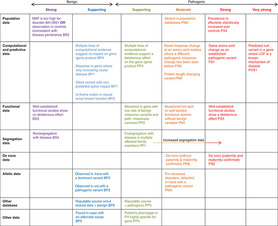
Standards and guidelines for the interpretation of sequence variants: a joint consensus recommendation of the American College of Medical Genetics and Genomics and the Association for Molecular Pathology

The ACMG/AMP framework uses five major classification categories:

Pathogenic
Likely pathogenic
Variant of uncertain significance (VUS)
Likely benign
Benign

The ACMG/AMP consensus recommendations describe evidence-based criteria incorporating population, computational, functional, segregation, and other evidence.

Why a VUS Is Not a Diagnosis

A Variant of Uncertain Significance means that available evidence is insufficient to confidently classify the variant as benign or pathogenic.

A VUS should therefore not automatically be interpreted as disease-causing.

This distinction is particularly important in clinical genetic testing.

The interpretation of variants can change as:

New studies are published
Population databases expand
Functional experiments become available
Clinical cases accumulate
Classification guidelines evolve

Therefore, variant interpretation is not necessarily static.

Evidence Used in Variant Interpretation

A clinical geneticist may consider:

Population evidence

Is the variant too common to cause the suspected disease?

Computational evidence

Do prediction tools suggest an effect on protein or splicing?

Functional evidence

Have laboratory experiments demonstrated a biological effect?

Segregation evidence

Does the variant track with disease within a family?

Allelic evidence

Are there other pathogenic variants in the same gene?

Phenotypic evidence

Does the patient’s phenotype match the known disease?

Literature evidence

Has the variant previously been described in affected individuals?

The ACMG/AMP framework integrates multiple evidence categories rather than relying on one computational prediction or one database entry.

Step 22: CNV Analysis

Not every important genomic alteration is a single nucleotide change.

Copy Number Variants (CNVs) involve changes in the number of copies of genomic regions.

Examples include:

Deletions
Duplications
Larger copy-number alterations

CNV analysis can be performed using:

Read-depth methods
Paired-end information
Split-read evidence
Specialized CNV callers
Platform-specific algorithms

For WES and targeted sequencing, read-depth analysis can be particularly useful.

A simplified model is:

Expected coverage
████████████████████

Observed coverage
████████

A significant reduction in read depth across a region may indicate a deletion, although technical and experimental factors must be considered.

Step 23: Structural Variant Analysis

Structural variants are larger genomic alterations.

Examples include:

Large deletions
Large insertions
Inversions
Translocations
Complex rearrangements

Short-read sequencing can detect some classes of structural variation, but detection sensitivity varies substantially depending on:

Variant size
Repetitive sequence
Breakpoint structure
Read length
Sequencing depth
Library design

Long-read sequencing can provide additional capabilities for resolving complex genomic regions.

Step 24: RNA-Seq Analysis

RNA-Seq requires a different analytical workflow because the goal is often to measure transcript abundance rather than directly identify genomic variants.

A simplified RNA-Seq pipeline is:

RNA Extraction
↓
RNA QC
↓
Library Preparation
↓
Sequencing
↓
FASTQ
↓
Read QC
↓
Trimming
↓
Alignment / Pseudoalignment
↓
Transcript Quantification
↓
Count Matrix
↓
Differential Expression
↓
Pathway / Functional Analysis

Depending on the research question, RNA-Seq may also be used for:

Alternative splicing
Fusion detection
Transcript discovery
Allele-specific expression
RNA editing
Isoform analysis

Differential Expression Analysis

In a typical RNA-Seq experiment, researchers may compare two or more biological conditions.

For example:

Control samples
        vs.
Disease samples

The analysis may identify genes that are:

Upregulated
Downregulated
Differentially expressed

Statistical models are used to account for:

Biological variation
Sequencing depth
Library size
Replicates
Experimental design

Importantly, biological replicates are essential for reliable differential expression analysis.

Step 25: Quality Control Should Continue Throughout the Pipeline

NGS QC is not a single step.

A robust pipeline contains multiple QC checkpoints.

Pre-sequencing QC

DNA/RNA concentration
Purity
Integrity
Library concentration
Fragment size

Raw-data QC

Read quality
GC distribution
Adapter content
Duplication
N content

Alignment QC

Mapping rate
Mapping quality
Proper pairing
Duplicate rate
Insert size

Coverage QC

Mean depth
Target coverage
Coverage uniformity
Low-coverage regions

Variant QC

Depth
Allele balance
Quality
Mapping evidence
Strand bias

This layered QC approach helps identify problems before they affect the final result.

Step 26: Reproducibility and Pipeline Management

A modern NGS pipeline should not simply produce a VCF file.

It should also preserve the information necessary to reproduce the analysis.

Important metadata include:

Reference genome version
Annotation version
Database versions
Software versions
Pipeline version
Parameters
Sample identifiers
Sequencing information
QC thresholds
Filtering criteria

For example:

Reference: GRCh38
Aligner: BWA-MEM2
Variant Caller: GATK HaplotypeCaller
Annotation: VEP
Population DB: gnomAD
Clinical DB: ClinVar
Pipeline Version: 2.4.1

Without this information, reproducing an old result can become difficult.

Workflow Automation

Large-scale NGS analysis involves many computational steps.

Manually executing every command is error-prone.

Modern pipelines therefore commonly use workflow management systems such as:

Nextflow
Snakemake
WDL
Cromwell
Workflow platforms
Cloud-based analysis systems

A workflow engine can define dependencies between steps.

For example:

FASTQ
↓
FastQC
↓
Trimming
↓
Alignment
↓
Sorting
↓
Duplicate Marking
↓
BQSR
↓
Variant Calling
↓
Filtering
↓
Annotation

If one stage fails, the workflow can often resume from the appropriate checkpoint rather than restarting the entire analysis.

Containers and Environment Reproducibility

Bioinformatics pipelines can depend on many software packages and system libraries.

Container technologies such as:

Docker
Singularity / Apptainer

can help standardize computational environments.

This reduces the risk of:

“It worked on one server but not on another.”

Containerized workflows are particularly valuable for:

Large research projects
Multi-user environments
Clinical pipelines
Cloud computing
Long-term reproducibility

Cloud-Based NGS Analysis

NGS generates very large datasets.

For example, a WGS project involving hundreds or thousands of samples can rapidly reach terabytes or petabytes of data.

Cloud computing can provide:

Elastic compute capacity
Large-scale storage
Parallel processing
Workflow orchestration
Data sharing
Scalable analysis

Cloud-based platforms can be particularly useful when computational requirements change significantly between projects.

GATK, for example, provides Best Practices workflows that can be run through cloud-based Terra workspaces.

Local vs Cloud NGS Analysis

There is no universally superior option.

Local infrastructure

Advantages:

Direct control of data
Predictable infrastructure
Existing HPC resources
Potentially economical at high utilization

Challenges:

Hardware maintenance
Storage management
Scaling
Software administration

Cloud infrastructure

Advantages:

Elastic scaling
No need to maintain physical servers
Rapid deployment
Parallel computing
Collaboration

Challenges:

Data transfer costs
Storage costs
Compute costs
Security configuration
Regulatory requirements

The appropriate model depends on project size, budget, infrastructure, data governance, and workload.

Clinical NGS vs Research NGS

Although the underlying technologies may be similar, clinical and research workflows have different requirements.

Research NGS

The primary goal may be:

Discovery
Hypothesis generation
Mechanistic research
Population analysis
Biomarker discovery

Researchers may have more flexibility in:

Pipeline design
Experimental methods
Exploratory analyses

Clinical NGS

Clinical analysis requires stronger emphasis on:

Analytical validity
Quality management
Traceability
Validation
Documentation
Interpretation
Reporting
Regulatory requirements

The ACMG/AMP recommendations emphasize standardized terminology and structured evidence-based interpretation for clinical sequence variant classification.

Therefore, a research pipeline should not automatically be treated as a clinically validated diagnostic pipeline.

Common NGS File Formats

Understanding file formats is essential for anyone working with NGS.

Format

Typical Purpose

FASTQ

Raw sequencing reads

SAM	Text alignment format

BAM	Binary alignment format

CRAM	Compressed alignment format

VCF	Variant calls

gVCF	Genomic variant representation for joint genotyping

BED	Genomic intervals

GTF/GFF

Gene/transcript annotation

BCL	Instrument-generated base-call data in relevant workflows

Each format represents a different stage of the workflow.

A Practical DNA NGS Pipeline

A simplified production-oriented germline pipeline may look like this:

Biological Sample
↓
DNA Extraction
↓
DNA QC
↓
Library Preparation
↓
Library QC
↓
Sequencing
↓
Raw Data
↓
Demultiplexing
↓
FASTQ
↓
Raw Read QC
↓
Adapter/Quality Processing
↓
Read Alignment
↓
BAM/CRAM
↓
Alignment QC
↓
Duplicate Marking
↓
Base Quality Processing
↓
Variant Calling
↓
VCF/GVCF
↓
Variant Filtering
↓
Variant Annotation
↓
Population Frequency Filtering
↓
Phenotype / Gene Prioritization
↓
Clinical or Biological Interpretation
↓
Final Report

GATK’s documented workflows follow this general conceptual structure, although the exact implementation, tools, and filtering models depend on the use case.

Example: WES Germline Analysis

Consider a patient undergoing WES for a suspected rare genetic disorder.

Step 1

DNA is extracted from the patient’s blood.

Step 2

DNA quality and concentration are evaluated.

Step 3

An exome library is prepared.

Step 4

The library is sequenced using paired-end sequencing.

Step 5

FASTQ files are generated.

patient_R1.fastq.gz
patient_R2.fastq.gz

Step 6

FastQC evaluates raw read quality.

Step 7

Reads are processed and aligned to GRCh38.

Step 8

An analysis-ready BAM/CRAM is generated.

Step 9

Germline variants are called.

Step 10

Variants are filtered.

Step 11

Variants are annotated with:

Gene
Transcript
Consequence
Population frequency
ClinVar information
Other evidence

Step 12

Variants are prioritized using:

Patient phenotype
Inheritance model
Gene-disease relationships
Population frequency
Variant consequence

Step 13

Candidate variants are manually reviewed.

Step 14

Relevant variants are interpreted according to appropriate clinical or research criteria.

Step 15

A final report is generated.

Example: Cancer NGS Workflow

Cancer sequencing has additional complexity.

A simplified tumor-normal workflow is:

Tumor Sample
↓
DNA Extraction
↓
Library Preparation
↓
Sequencing
↓
FASTQ
↓
QC
↓
Alignment
↓
BAM
↓
Somatic Calling
↓
Variant Filtering
↓
VAF / CNV / SV
↓
Annotation
↓
Clinical Interpretation

Somatic analysis may need to consider:

Tumor purity
Normal contamination
VAF
Copy number
Tumor heterogeneity
Germline background
Matched normal sample
Panel of normals
Cancer-specific databases

Common NGS Analysis Challenges

Even a technically sophisticated sequencing experiment can produce misleading results if the analytical workflow is poorly designed.

Common challenges include:

Low sequencing quality

Can reduce confidence in variant calls.

Poor coverage

Can create false-negative risks.

PCR duplicates

Can distort allele representation.

Mapping ambiguity

Can cause incorrect variant assignment.

Reference genome mismatch

Can make coordinates and annotations inconsistent.

Incorrect transcript selection

Can change HGVS representation and predicted consequences.

Outdated databases

Can lead to incomplete interpretation.

Incorrect filtering

Can remove true variants or retain artifacts.

Sample contamination

Can create unexpected allele frequencies and false calls.

Sample swaps

Can result in completely incorrect conclusions.

Pipeline inconsistency

Changing tools or parameters between samples can introduce batch effects.

False Positives and False Negatives

NGS analysis must balance two major classes of errors.

False Positive

A variant is reported even though it is not truly present.

Potential causes include:

Sequencing errors
Alignment artifacts
PCR artifacts
Contamination
Low mapping quality
Incorrect variant modeling

False Negative

A real variant is not detected.

Potential causes include:

Insufficient coverage
Poor mapping
Difficult genomic regions
Low variant allele fraction
Inadequate caller sensitivity
Structural complexity
Reference bias

Therefore, variant calling should always be interpreted together with QC and coverage information.

Why One NGS Pipeline Cannot Detect Everything

Different variant classes require different analytical strategies.

A pipeline optimized for SNVs and small indels may not reliably detect:

Large structural variants
Repeat expansions
Complex rearrangements
Certain CNVs
Deep intronic variants
Difficult repetitive regions

Similarly, a WES pipeline cannot provide the same genomic information as WGS because much of the non-coding genome is not directly targeted.

This is why test selection and pipeline design must be aligned with the biological question.

Manual Review of Candidate Variants

Automated pipelines are extremely powerful, but candidate variants may still require manual review.

Genome browsers such as IGV can be used to inspect:

Read depth
Variant allele balance
Mapping quality
Strand distribution
Nearby indels
Alignment patterns
Potential sequencing artifacts

A candidate variant that appears convincing in a VCF may look suspicious when viewed at the read level.

Therefore: Automated analysis identifies candidates; evidence-based review determines their relevance.

What Does a Good NGS Pipeline Look Like?

A robust NGS pipeline should be:

Accurate

It should reliably identify the intended variant classes.

Reproducible

The same input and pipeline configuration should produce consistent results.

Scalable

It should work for one sample as well as large cohorts.

Traceable

Software versions, references, databases, and parameters should be recorded.

Auditable

Every analytical step should be inspectable.

Validated

Performance should be evaluated against appropriate reference datasets.

Automated

Manual intervention should be minimized where appropriate.

Transparent

QC metrics and filtering decisions should be visible to the user.

What Is an NGS Analysis Pipeline?

An NGS pipeline is a structured sequence of computational operations that transforms sequencing data into a final analytical result.

For example:

FASTQ
↓
Quality Control
↓
Trimming
↓
Alignment
↓
BAM Processing
↓
Variant Calling
↓
Variant Filtering
↓
Annotation
↓
Prioritization
↓
Interpretation

The important distinction is that a pipeline is not simply a list of software tools.

A production-quality pipeline also defines:

Input requirements
Output formats
Parameters
Quality thresholds
Reference versions
Database versions
Error handling
Logging
Reproducibility
QC criteria

Example NGS Tools by Workflow Stage

Workflow Stage

Common Tools / Technologies

Raw QC

FastQC

QC aggregation

MultiQC

Adapter trimming

Cutadapt, fastp, Trimmomatic

Alignment

BWA-MEM2, DRAGMAP

Alignment processing

SAMtools, Picard

Variant calling

GATK HaplotypeCaller, Mutect2 and others

Variant annotation

Ensembl VEP, SnpEff

Clinical annotation

ClinVar and other resources

Visualization

IGV

Workflow management

Nextflow, Snakemake, WDL

Cloud execution

Terra and other cloud platforms

The optimal toolset depends on the sequencing platform, assay, variant type, and validation requirements.

NGS Analysis Is an End-to-End Process

One of the most common misconceptions is that NGS analysis begins when FASTQ files are received.

In reality, data quality is influenced from the earliest stages of the experiment.

A more accurate representation is:

Sample Quality
↓
Library Quality
↓
Sequencing Quality
↓
Read Quality
↓
Alignment Quality
↓
Coverage Quality
↓
Variant Quality
↓
Annotation Quality
↓
Interpretation Quality
↓
Final Result

An error introduced early in the workflow can propagate through every downstream stage.

The Importance of Reference and Database Versioning

Suppose two analyses use:

GRCh38

but different annotation releases.

The resulting annotations may differ.

Likewise, a variant classification in ClinVar may change over time as new evidence is submitted.

ClinVar itself is continuously updated and provides information about submissions, interpretations, conditions, and supporting evidence.

Therefore, a reproducible NGS report should ideally record:

Genome assembly
Annotation release
Database release
Pipeline version
Tool versions
Analysis date

From Raw Data to Biological Knowledge

The NGS workflow can be understood as a series of transformations:

Level 1 – Biological material

Blood / Tissue / Cells

Level 2 – Sequencing library

DNA/RNA → Sequencing Library

Level 3 – Raw sequencing data

Library → FASTQ

Level 4 – Aligned data

FASTQ → BAM/CRAM

Level 5 – Variant or expression data

BAM/CRAM → VCF / Count Matrix

Level 6 – Annotated data

VCF → Annotated Variants

Level 7 – Biological interpretation

Annotated Variants
↓
Prioritized Candidates
↓
Biological / Clinical Interpretation

This final transformation is the real purpose of NGS analysis.

Key Takeaways

A complete NGS analysis workflow involves substantially more than sequencing.

The major stages are:

Define the biological question
Select the appropriate sequencing strategy
Collect and prepare the sample
Extract DNA or RNA
Perform nucleic acid QC
Prepare sequencing libraries
Perform library QC
Sequence the libraries
Generate raw sequencing data
Perform raw read QC
Remove adapters and process low-quality reads when appropriate
Align reads or quantify transcripts
Perform alignment QC
Generate analysis-ready files
Call variants or quantify expression
Filter low-confidence results
Annotate variants
Integrate population and clinical databases
Prioritize candidate variants
Interpret the biological or clinical significance
Review relevant findings
Generate the final report
Preserve metadata for reproducibility

The most important principle is that NGS analysis is an end-to-end workflow. High-quality sequencing data alone do not guarantee high-quality biological conclusions.

A reliable NGS result requires appropriate experimental design, robust quality control, validated computational methods, accurate annotation, and evidence-based interpretation.

For research and clinical applications alike, the ultimate objective is not to produce the largest possible number of variants. It is to transform sequencing data into accurate, reproducible, interpretable, and biologically meaningful information.

References and Further Reading

Illumina – NGS Workflow Steps
Overview of nucleic acid extraction, library preparation, sequencing, and the general NGS workflow.
GATK – Best Practices Workflows
Comprehensive documentation covering germline, somatic, structural variant, mitochondrial, RNA-Seq and preprocessing workflows.
GATK – Data Pre-processing for Variant Discovery
Documentation covering alignment and preprocessing of sequencing data to produce analysis-ready BAM files.
GATK – Germline Short Variant Discovery
Documentation for germline SNP and indel discovery, including GVCF generation and joint genotyping.
GATK – Somatic Short Variant Discovery
Documentation describing somatic SNV and indel discovery and filtering workflows.
GATK – HaplotypeCaller
Technical explanation of active-region detection, local reassembly and haplotype-based variant calling.
FastQC – Babraham Bioinformatics
Quality-control tool and documentation for high-throughput sequencing data.
NCBI – FASTQ File Format Guide
Documentation describing FASTQ structure, sequence data and per-base quality scores.
Ensembl – Variant Effect Predictor (VEP)
Documentation for predicting the effects of variants on genes, transcripts, proteins and regulatory regions.
NCBI – ClinVar
Public archive of relationships between human genomic variation and diseases or drug responses, including supporting evidence.
Richards et al. – ACMG/AMP Sequence Variant Interpretation Guidelines
Richards S, Aziz N, Bale S, et al. Standards and guidelines for the interpretation of sequence variants: a joint consensus recommendation of the American College of Medical Genetics and Genomics and the Association for Molecular Pathology. Genetics in Medicine. 2015;17(5):405–424.
Landrum et al. – ClinVar
Landrum MJ, Lee JM, Riley GR, et al. ClinVar: public archive of relationships among sequence variation and human phenotype. Nucleic Acids Research. 2014;42(Database issue):D980–D985.

Final Perspective

NGS has made it possible to interrogate genomic and transcriptomic information at an unprecedented scale. But the sequencing instrument is only one component of the overall system.

The real analytical value emerges when high-quality sequencing data are combined with:

quality control + bioinformatics + variant detection + annotation + biological context + evidence-based interpretation.

A well-designed NGS workflow therefore connects the laboratory and computational worlds into a single reproducible process—from the original biological sample to a result that researchers, geneticists, clinicians, and other specialists can meaningfully interpret.