What Is an NGS Analysis Pipeline and How to Build One?

Next-Generation Sequencing (NGS) has become one of the fundamental technologies in genomics, molecular diagnostics, and biomedical research by making it possible to sequence millions or even billions of DNA or RNA molecules in a relatively short period of time. However, raw sequencing data generated by an NGS instrument is not, by itself, a biologically or clinically meaningful result. The raw sequencing output must pass through a series of computational processes, including quality control, read preprocessing, reference genome alignment, variant calling, variant filtering, annotation, prioritization, and interpretation. The systematic and automated execution of these processes is referred to as an NGS analysis pipeline.

In its simplest definition:

An NGS pipeline is an automated computational workflow that transforms raw sequencing data into reliable, reproducible, traceable, and biologically or clinically interpretable results.

A typical DNA-sequencing workflow may begin with FASTQ files, proceed through quality control and optional trimming, align reads to a reference genome, generate BAM/CRAM files, identify variants, filter them, annotate them, and finally support biological or clinical interpretation. Illumina similarly describes NGS data analysis as a sequence of processes beginning with raw sequencing data and FASTQ generation, followed by quality control, alignment, variant calling or quantification, and downstream biological interpretation.

However, an NGS pipeline is much more than a collection of commands executed sequentially. A production-grade pipeline should:

• address a clearly defined biological or clinical question,
• use appropriate computational tools,
• perform quality control at multiple stages,
• handle errors safely,
• document software and reference versions,
• provide reproducible results,
• scale from individual samples to large cohorts,
• maintain complete provenance,
• support reruns and partial recovery,
• and, when used clinically, undergo appropriate analytical validation.

Therefore, a high-quality NGS pipeline should be viewed not merely as a script, but as a software system combining molecular biology, bioinformatics, data engineering, computational infrastructure, and quality management.

What Is an NGS Pipeline?

An NGS pipeline is a structured workflow that processes sequencing data through a predefined sequence of computational steps.

For example, a simplified germline DNA-sequencing pipeline may look like this:

Sequencer
↓
Raw Data
↓
FASTQ
↓
Raw QC
↓
Trimming / Filtering
↓
Alignment
↓
BAM / CRAM
↓
Post-alignment QC
↓
Variant Calling
↓
Variant Filtering
↓
Variant Annotation
↓
Clinical / Biological Interpretation
↓
Report

However, real-world pipelines are not necessarily linear.

For example:

                         ┌── SNV / Indel Calling ──┐
FASTQ → QC → Alignment ──┼── CNV Calling ──────────┼→ Annotation
                         ├── SV Calling ───────────┤
                         └── Mitochondrial Calling┘
                                      ↓
                                  Filtering
                                      ↓
                                Interpretation
                                      ↓
                                   Report

This type of architecture allows a single sequencing dataset to be analyzed for multiple classes of genomic variation.

Are Pipeline and Workflow the Same Thing?

The terms pipeline, workflow, analysis workflow, and bioinformatics pipeline are frequently used interchangeably in genomics. Nevertheless, it is useful to distinguish them conceptually.

Workflow

A workflow describes the logical sequence of analytical operations.

For example:

FASTQ
↓
QC
↓
Alignment
↓
Variant Calling
↓
Annotation

Pipeline

A pipeline is the implementation of that workflow using actual software tools, parameters, dependencies, input/output definitions, and execution logic.

For example:

FastQC
↓
fastp
↓
BWA-MEM2
↓
Samtools
↓
GATK
↓
VEP

Workflow Engine

A workflow engine manages how these processes are executed, including dependencies, parallelization, resource allocation, retries, and workflow state.

Examples include:

• Nextflow
• Snakemake
• WDL + Cromwell
• Galaxy
• CWL-based systems

Workflow engines become particularly important when pipelines need to process large numbers of samples or operate in production environments.

Why Are NGS Pipelines Necessary?

NGS experiments can generate millions or billions of sequencing reads. In whole-genome sequencing, the resulting data may consist of hundreds of gigabytes of raw and intermediate files.

Manually processing such datasets is impractical, error-prone, and difficult to reproduce.

The major purposes of an NGS pipeline are therefore:

Automation

The same analytical procedures can be applied automatically to every sample.

Standardization

The same:

• tools,
• software versions,
• parameters,
• reference genomes,
• annotation resources,
• filtering rules

can be consistently applied.

Reproducibility

An analysis can be rerun using the same inputs and computational environment.

Scalability

A pipeline can process one sample or thousands of samples using the same workflow architecture.

Traceability

It should be possible to determine which:

• pipeline version,
• tool version,
• reference genome,
• database version,
• parameter set

was used to generate a particular result.

Error Detection

Quality-control checkpoints can identify problems before they propagate through downstream analysis.

Resource Management

CPU, RAM, storage, and, where applicable, GPU resources can be allocated according to the requirements of each process.

What Makes a Good NGS Pipeline?

A good pipeline must do more than simply produce an output file.

Important characteristics include:

Characteristic	Description

Accuracy

Produces biologically and analytically correct results

Reproducibility

Produces consistent results under controlled conditions

Traceability

Allows results to be traced back to their processing steps

Scalability

Can process increasing numbers of samples

Robustness

Handles unexpected conditions safely

Maintainability

Can be updated without excessive redevelopment

Portability

Can operate across different computing environments

Testability

Individual components can be independently tested

Auditability

Processing history can be reviewed

Performance

Uses computational resources efficiently

For clinical applications, these requirements become particularly important.

The First Step: Define the Purpose of the Pipeline

Before selecting any software, the most important question is:

What biological or clinical question is the pipeline supposed to answer?

There is no universal “NGS pipeline.”

Different workflows are required for:

• Whole Genome Sequencing (WGS)
• Whole Exome Sequencing (WES)
• targeted gene panels
• hereditary cancer analysis
• somatic cancer analysis
• NIPT
• RNA-seq
• single-cell RNA-seq
• methylation sequencing
• metagenomics
• microbiome analysis
• pharmacogenomics
• mitochondrial sequencing
• CNV analysis
• structural variant analysis

GATK’s Best Practices similarly emphasizes that workflows depend on the experimental design, sequencing technology, data type, and type of variation being investigated.

Define the Sequencing Data Type

The second major design decision is identifying the type of sequencing data.

Whole Genome Sequencing

WGS covers the entire genome and can potentially provide information about:

• coding regions,
• non-coding regions,
• SNVs,
• indels,
• CNVs,
• structural variants,
• mitochondrial variants.

The major disadvantage is the large computational and storage requirement.

Whole Exome Sequencing

WES focuses primarily on protein-coding regions.

Important QC metrics include:

• mean/median target coverage,
• percentage of targets above a defined depth,
• target enrichment,
• on-target rate,
• off-target reads,
• coverage uniformity.

Targeted Panels

Targeted sequencing focuses on specific genes, regions, or known hotspots.

Important metrics often include:

• high sequencing depth,
• target coverage,
• hotspot coverage,
• coverage uniformity,
• on-target percentage.

RNA-seq

RNA-seq requires a substantially different workflow from DNA sequencing.

A typical RNA-seq workflow is:

FASTQ
↓
QC
↓
Trimming
↓
Splice-aware Alignment
↓
BAM
↓
Transcript Quantification
↓
Gene Expression
↓
Differential Expression
↓
Pathway Analysis

RNA-seq workflows must account for transcript structure, exon-exon junctions, alternative splicing, and transcript isoforms. Consequently, splice-aware aligners and RNA-specific downstream analyses are required.

Define Pipeline Inputs and Outputs

Before implementation, all inputs and outputs should be explicitly defined.

For example, a germline WES pipeline may use:

Input

sample_R1.fastq.gz
sample_R2.fastq.gz
reference.fasta
target_regions.bed

Intermediate Outputs

trimmed_R1.fastq.gz
trimmed_R2.fastq.gz
aligned.bam
aligned.bam.bai
recalibrated.bam

Final Outputs

variants.vcf.gz
variants.vcf.gz.tbi
annotated.vcf.gz
qc_report.html
analysis_report.html

This separation is fundamental to good pipeline architecture.

The Major Stages of an NGS Pipeline

A typical DNA-sequencing pipeline can be divided into several major analytical stages.

Stage 1: Raw Data Acquisition

The first step is obtaining sequencing data from the sequencing platform.

Depending on the sequencing technology and instrument, different intermediate formats may be generated. In many Illumina-based workflows, sequencing data are processed into FASTQ files for downstream analysis.

The most common input format is:

FASTQ

For paired-end sequencing, files may look like:

SAMPLE_R1.fastq.gz
SAMPLE_R2.fastq.gz

where:

• R1 represents the first read,
• R2 represents the second read.

A FASTQ record typically contains:

@READ_ID
ACTGACTGACTG
+
FFFFFFFFFFFF

The four lines represent:

1. read identifier,
2. nucleotide sequence,
3. separator,
4. base quality scores.

FASTQ Quality Scores

Base quality scores are essential for assessing sequencing reliability.

The Phred quality score is defined as:

[
Q = -10 \log_{10}(P_e)
]

where:

• (Q) is the Phred quality score,
• (P_e) is the probability of an incorrect base call.

For example:

Phred Score

Error Probability

Q10

10%

Q20

1%

Q30

0.1%

Q40

0.01%

Thus, a Q30 base has an estimated error probability of approximately 0.1%.

Stage 2: Initial Quality Control

The first analytical checkpoint is usually raw sequencing QC.

The goal is to answer:

Is this sequencing dataset of sufficient quality to proceed with downstream analysis?

Common tools include:

• FastQC
• MultiQC
• fastp
• FastQ Screen
• Falco

Galaxy Training Network materials similarly emphasize the importance of preprocessing and quality assessment before downstream mapping and variant analysis.

What Should Be Evaluated During FASTQ QC?

Per-base Sequence Quality

This examines quality scores across sequencing cycles.

A decline in quality toward the end of reads is common in some sequencing datasets.

Per-sequence Quality

This evaluates the overall quality distribution across reads.

GC Content

Unexpected GC distributions can indicate:

• library bias,
• contamination,
• amplification bias,
• unusual sequence composition.

Sequence Duplication

High duplication can indicate:

• PCR amplification,
• low library complexity,
• technical artifacts.

However, duplication is not inherently bad.

Targeted sequencing and amplicon-based assays can naturally exhibit high duplication.

Adapter Contamination

The presence of adapter sequences should be evaluated.

Overrepresented Sequences

Unexpectedly abundant sequences may indicate:

• adapter contamination,
• technical artifacts,
• contamination,
• biological features specific to the sample.

QC-Based Decision Making

A production pipeline should not simply perform QC and continue automatically.

A better architecture is:

             FASTQ
               ↓
              QC
               ↓
       ┌───────┴────────┐
       ↓                ↓
     PASS              FAIL
       ↓                ↓
 Continue         Stop / Review

A more sophisticated system may use:

QC
 ↓
 ├── PASS → Continue
 ├── WARNING → Continue + Flag
 └── FAIL → Stop

The exact thresholds should be determined through assay-specific validation.

Stage 3: Adapter Trimming and Read Filtering

If required, adapter sequences and low-quality bases can be removed.

Common tools include:

• fastp
• Cutadapt
• Trimmomatic

Typical operations include:

• adapter removal,
• quality trimming,
• minimum read-length filtering,
• low-quality base removal.

However, trimming should not automatically be included in every pipeline.

The decision depends on:

• sequencing platform,
• assay design,
• read quality,
• downstream tools,
• validation results.

Overly aggressive trimming can shorten reads unnecessarily and potentially affect mapping or variant detection.

Stage 4: Alignment

After preprocessing, reads are aligned to a reference genome.

The purpose is to determine the most likely genomic location of each sequencing read.

For example:

Read:
ATCGATCGATCG

Reference:
...ATCGATCGATCG...
       ↑
    alignment

Common alignment tools include:

• BWA-MEM2
• Bowtie2
• minimap2
• STAR
• HISAT2

BWA-based alignment has historically been an important component of short-read DNA sequencing workflows, including the GATK Best Practices framework.

Reference Genome Selection

The reference genome is one of the most critical components of an NGS pipeline.

For human genomic analysis, commonly encountered builds include:

• GRCh37 / hg19
• GRCh38 / hg38

However, selecting a FASTA file is not sufficient.

Associated resources must also be compatible with the same genome build, including:

• FASTA,
• FASTA index,
• sequence dictionary,
• annotation resources,
• known-sites resources,
• dbSNP,
• BED files,
• transcript databases.

For example:

GRCh38 FASTA
+
GRCh37 BED

is an incompatible combination that can produce serious analytical errors.

Therefore, genome build information must be explicitly tracked throughout the pipeline.

Alignment Output: SAM, BAM, and CRAM

Alignment results may initially be represented in:

SAM

format.

For efficient storage and processing, alignment data are commonly converted to:

BAM

or:

CRAM

BAM stands for Binary Alignment/Map.

CRAM provides a more compact representation and can reduce storage requirements for large sequencing datasets.

Stage 5: Post-alignment QC

Alignment must also be followed by quality assessment.

Important metrics may include:

• mapping rate,
• properly paired reads,
• duplicate rate,
• mean depth,
• median depth,
• insert size,
• mapping quality,
• target coverage,
• coverage uniformity,
• on-target rate.

For example:

Total Reads          : 120,000,000
Mapped Reads         : 117,500,000
Mapping Rate         : 97.9%
Duplicate Rate       : 8.2%
Mean Coverage        : 125X

These metrics help determine whether the sequencing data are suitable for downstream variant analysis.

Why Is Coverage Important?

Coverage refers to the number of sequencing reads supporting a genomic position.

For example:

Position 1001 → 50 reads
Position 1002 → 52 reads
Position 1003 → 3 reads

Position 1003 has substantially lower coverage.

Low coverage can increase the risk of:

• false negatives,
• low-confidence calls,
• allelic dropout,
• incomplete target assessment.

For clinical sequencing, mean depth alone is therefore insufficient.

Mean Coverage Alone Is Not Enough

Consider two samples:

Sample A:
Mean depth = 100X
95% of targets >20X

and:

Sample B:
Mean depth = 100X
65% of targets >20X

Both have the same mean depth, but their effective coverage profiles are very different.

Therefore, WES and targeted-panel pipelines should evaluate coverage distributions and the percentage of target bases above relevant thresholds.

Stage 6: BAM Processing

Depending on the workflow, alignment data may undergo:

• sorting,
• duplicate marking,
• base quality score recalibration,
• read-group assignment,
• indexing.

GATK’s Best Practices framework separates data preprocessing from variant discovery and emphasizes the generation of analysis-ready alignment files before variant calling.

Read Groups

Read-group information is important for downstream analysis.

Common fields include:

ID
SM
LB
PL
PU

These fields can describe:

• sample,
• library,
• sequencing platform,
• sequencing unit.

Incorrect sample metadata can lead to serious downstream errors even if the computational pipeline itself runs successfully.

Duplicate Marking

PCR amplification and sequencing processes can generate duplicate reads.

Duplicate marking is commonly performed in:

• WGS,
• WES,
• targeted sequencing.

However, duplicates should not automatically be interpreted as meaningless.

For example, high duplication may be expected in:

• amplicon sequencing,
• ultra-deep sequencing,
• highly targeted assays.

Therefore, duplicate rates must always be interpreted in the context of assay design.

Base Quality Score Recalibration

Base Quality Score Recalibration (BQSR) aims to recalibrate sequencing quality scores using known technical and contextual patterns.

The objective is to improve the reliability of base-quality estimates used by downstream variant calling algorithms.

The exact preprocessing steps should always be aligned with the requirements of the selected variant caller and the overall validated workflow.

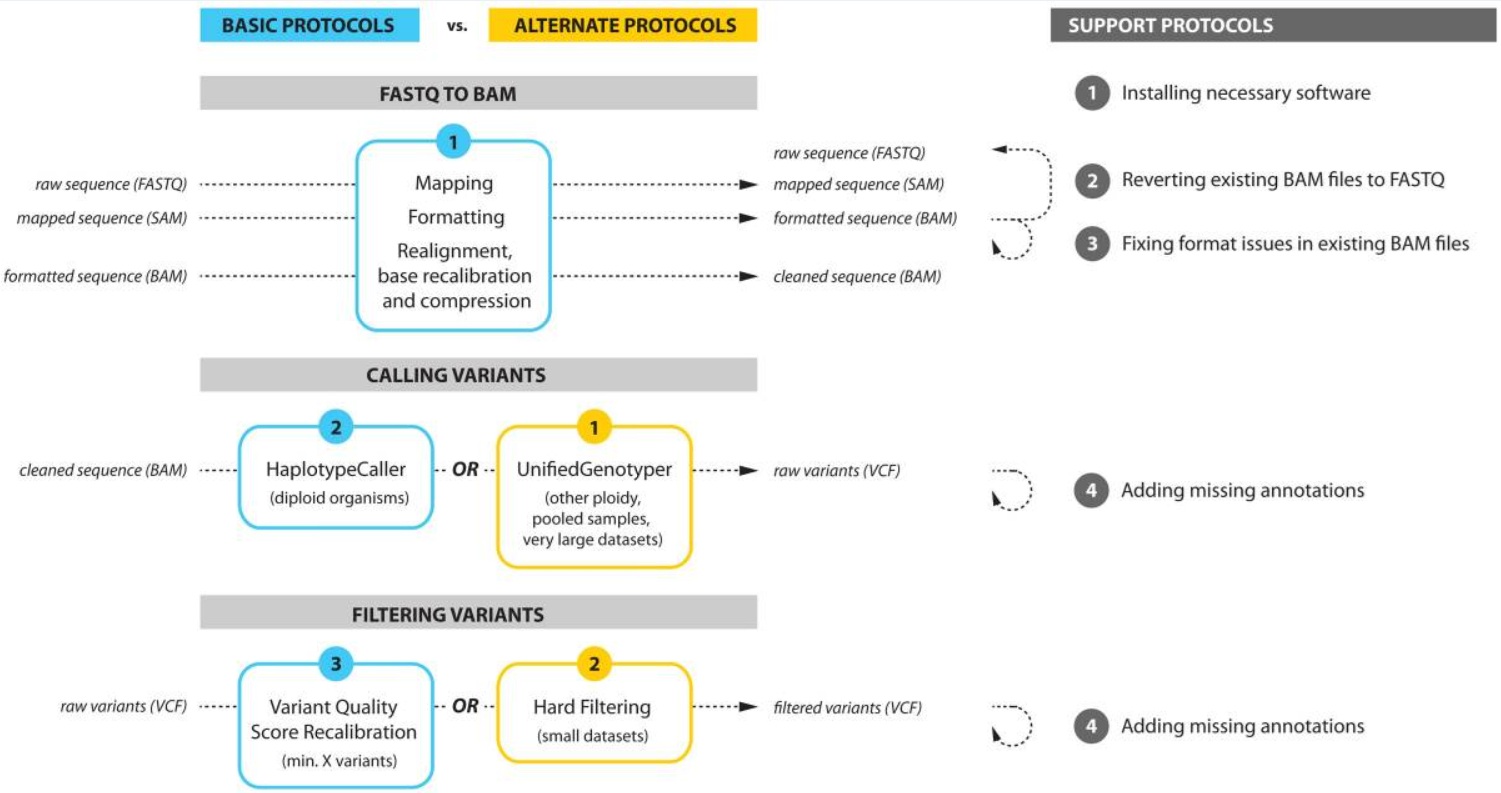
Stage 7: Variant Calling

After alignment, the fundamental question becomes:

Which genomic positions differ between the sample and the reference genome?

This process is known as variant calling.

Variant calling identifies genomic positions that differ from the reference.

Genotype calling then determines the genotype represented by the sample at those positions.

Galaxy Training Network explicitly distinguishes variant calling from genotype determination and provides dedicated workflows for these processes.

Types of Variants

A pipeline should define which variant classes it is designed to detect.

SNVs

Single Nucleotide Variants involve a single nucleotide difference.

For example:

Reference: A
Sample:    G

Small Insertions and Deletions

Small insertions and deletions are generally referred to as indels.

For example:

Reference:
ATCGATCG

Sample:
ATCGCG

Copy Number Variants

CNVs represent changes in the number of copies of a genomic region.

For example:

Normal:
2 copies

Sample:
1 copy

or:

Normal:
2 copies

Sample:
4 copies

Structural Variants

Structural variants include larger genomic alterations such as:

• deletions,
• duplications,
• inversions,
• translocations.

Mitochondrial Variants

Mitochondrial DNA has distinct biological and computational properties and may therefore require a dedicated analysis branch.

Germline Variant Calling

Germline analysis aims to identify inherited genetic variation.

A simplified workflow is:

FASTQ
↓
QC
↓
Alignment
↓
BAM
↓
Germline Variant Caller
↓
GVCF / VCF
↓
Genotyping
↓
Filtering
↓
Annotation

GATK provides a dedicated Best Practices framework for germline short-variant discovery.

Somatic Variant Calling

Somatic analysis is particularly important in cancer genomics.

The typical tumor-normal workflow is:

Tumor FASTQ ─────┐
                 ├→ Alignment
Normal FASTQ ────┘
                       ↓
                Tumor BAM
                Normal BAM
                       ↓
                Somatic Caller
                       ↓
                 Somatic VCF

Tumor-only workflows are also possible.

Somatic variant analysis must account for factors such as:

• variant allele fraction,
• tumor purity,
• normal contamination,
• sequencing depth,
• strand bias,
• mapping artifacts.

GATK provides separate somatic variant discovery workflows rather than treating somatic calling as a simple extension of germline analysis.

Why Is CNV Calling Different?

SNV/indel calling and CNV detection are fundamentally different computational problems.

CNV detection can rely on signals such as:

• read depth,
• segmentation,
• allele-specific information,
• B-allele frequency,
• normalization.

Therefore:

SNV/Indel branch

and:

CNV branch

should generally be treated as separate components.

Structural Variant Analysis

Structural variant detection can use signals such as:

• split reads,
• discordant read pairs,
• read-depth changes,
• local assembly.

Consequently, a WGS pipeline may contain multiple variant-detection branches:

                         ┌── SNV / Indel
                         │
FASTQ → QC → Alignment ──┼── CNV
                         │
                         ├── SV
                         │
                         └── Mitochondrial

GATK-SV also provides dedicated workflows and quality-control approaches for structural variation analysis.

Stage 8: Variant Filtering

Variant callers may produce large numbers of candidate variants, many of which are not biologically meaningful.

For example:

Total variants:
4,500,000

may include:

• sequencing artifacts,
• mapping artifacts,
• low-quality calls,
• insufficient-depth calls,
• low allele-fraction calls,
• common benign variants.

Filtering is therefore essential.

Hard Filtering

Hard filtering applies explicit thresholds.

For example:

DP >= 20
QUAL >= 30
MQ >= 40
VAF >= 0.20

However, these thresholds are not universal.

A threshold appropriate for a highly targeted panel may be inappropriate for WGS.

Filtering thresholds should therefore be established according to:

• assay design,
• sequencing platform,
• coverage,
• variant caller,
• biological question,
• validation data.

Variant Quality Score Recalibration

Variant Quality Score Recalibration (VQSR) uses statistical modeling to distinguish higher-confidence from lower-confidence variant calls.

Rather than relying solely on a single threshold such as:

QUAL > X

multiple variant-level features can be modeled.

However, the suitability of VQSR depends on factors such as dataset size and the availability of appropriate training and truth resources.

Therefore, methods designed for large WGS/WES datasets should not automatically be applied to small targeted panels.

Stage 9: Variant Annotation

A raw VCF record such as:

chr7:140453136 A>T

does not, by itself, explain the biological or clinical significance of the variant.

Annotation adds information such as:

• gene,
• transcript,
• exon,
• cDNA change,
• protein change,
• molecular consequence,
• population frequency,
• clinical significance,
• disease association.

Annotation Databases and Resources

Depending on the analytical objective, resources may include:

• ClinVar
• dbSNP
• gnomAD
• OMIM
• COSMIC
• dbNSFP
• Ensembl
• RefSeq
• HGMD

The version of each database is as important as the database itself.

For example:

ClinVar:
specific release date/version

gnomAD:
specific release

Reference:
GRCh38

Transcript:
MANE Select

This information should be preserved as part of the analysis provenance.

Annotation Is Not Interpretation

This distinction is particularly important in clinical genomics.

Annotation

Adds information to a variant.

For example:

Gene: BRCA1
Consequence: missense_variant
Population AF: 0.0001
ClinVar: Pathogenic

Interpretation

Evaluates that information in the context of:

• patient phenotype,
• inheritance,
• clinical evidence,
• functional evidence,
• population data,
• literature,
• disease mechanism.

Therefore:

Annotation ≠ Interpretation

An annotation engine provides evidence. It does not automatically replace expert clinical interpretation.

ACMG/AMP Variant Classification

The ACMG/AMP framework is widely used for germline variant interpretation.

Variants can generally be classified into categories such as:

• Pathogenic
• Likely Pathogenic
• Variant of Uncertain Significance
• Likely Benign
• Benign

An important distinction is:

A variant caller reporting PASS does not mean that the variant is clinically pathogenic.

Similarly:

The presence of a pathogenic classification in a database does not automatically mean that a variant can be interpreted without considering the specific clinical context.

Variant Prioritization

A WES or WGS dataset can contain thousands or millions of variants.

A prioritization workflow may look like:

All Variants
↓
Quality Filtering
↓
Population Frequency
↓
Functional Consequence
↓
Gene Panel
↓
Disease Association
↓
Phenotype
↓
Candidate Variants

This reduces the candidate space for detailed review.

Phenotype-driven Analysis

Clinical genomic pipelines can incorporate phenotype information.

For example:

Patient Phenotype
↓
HPO Terms
↓
Candidate Genes
↓
Candidate Variants
↓
Ranking

This approach is especially useful in rare-disease diagnostics.

QC Should Exist at Multiple Levels

A professional pipeline should not rely on a single QC step.

At minimum, QC should be considered at:

Raw Data QC

FASTQ
↓
QC

Alignment QC

BAM
↓
Mapping / Coverage QC

Variant QC

VCF
↓
Variant QC

In clinical workflows, an additional interpretation/reporting QC layer may also be appropriate.

How Should QC Thresholds Be Defined?

One of the most common mistakes is copying arbitrary thresholds from another pipeline.

For example:

Q30 > 80%

may be useful in one assay but inappropriate in another.

Threshold development should consider:

1. assay design,
2. sequencing platform,
3. library preparation,
4. sample type,
5. coverage distribution,
6. validation datasets,
7. known positive and negative samples.

Clinical QC thresholds should be supported by analytical validation.

Error Handling

A production pipeline must define what happens when something goes wrong.

For example:

FASTQ missing

or:

Reference index missing

or:

BAM empty

or:

QC failed

or:

Disk full

or:

Tool crashed

A robust architecture may behave like:

QC FAIL
↓
Pipeline STOP
↓
Error Log
↓
Notification

A pipeline should never silently continue and generate apparently valid output after a critical upstream failure.

Logging

Every major process should produce logs.

For example:

2026-08-20 12:31:10
Sample: SAMPLE001
Process: Alignment
Tool: BWA-MEM2
Version: X.X
Reference: GRCh38
Status: STARTED

followed by:

2026-08-20 12:48:21
Sample: SAMPLE001
Process: Alignment
Status: COMPLETED
Exit code: 0

Logging is essential for:

• troubleshooting,
• monitoring,
• auditing,
• reproducibility.

Metadata Management

The pipeline should manage metadata in addition to sequencing files.

Possible fields include:

sample_id
patient_id
library_id
platform
run_id
read_group
sample_type
tumor_normal
sex
batch
reference
pipeline_version

In clinical systems, the distinction between sample identifiers and patient identifiers is particularly important.

Pipeline Versioning

Suppose an analysis was performed using:

Pipeline v1.0

and six months later the pipeline has become:

Pipeline v2.0

The same FASTQ files may produce different results.

Therefore, every result should retain:

Pipeline Version
Tool Versions
Reference Version
Database Versions
Parameters

GATK’s documentation also emphasizes that workflows and recommended methods evolve over time, meaning that simply stating that a pipeline “uses GATK” is insufficient to describe its computational environment.

A better description is:

GATK version X.X was used with reference genome Y, resource set Z, and the specified parameters.

Software Versioning

For example:

BWA-MEM2: X.X
Samtools: X.X
GATK: X.X
VEP: X.X

should be recorded.

This becomes critical when troubleshooting differences between historical and current analyses.

Containerization

Container technologies can improve reproducibility by packaging software and dependencies together.

Common technologies include:

• Docker
• Singularity
• Apptainer

A container can package:

Tool
+
Libraries
+
Dependencies
+
Operating environment

into a controlled computational environment.

This reduces the risk that a pipeline behaves differently because of differences in system libraries or software installations.

Choosing a Workflow Engine

A small pipeline can technically be implemented using shell scripts:

fastqc sample.fastq.gz
bwa-mem2 mem reference.fa sample.fastq.gz > sample.sam
samtools sort sample.sam -o sample.bam
gatk HaplotypeCaller -I sample.bam -O sample.vcf

However, this approach becomes difficult to maintain as the pipeline grows.

Production workflows often require:

• dependency management,
• parallelization,
• retries,
• resume capability,
• resource management,
• logging,
• metadata tracking,
• workflow visualization.

This is where workflow engines become valuable.

Nextflow

Nextflow is a widely used workflow management framework in bioinformatics.

A workflow might conceptually look like:

FASTQ
↓
QC
↓
Alignment
↓
BAM
↓
Variant Calling
↓
VCF
↓
Annotation

Nextflow can manage:

• process dependencies,
• data channels,
• parallelization,
• execution environments,
• containers,
• cloud/HPC execution,
• workflow resumption.

The nf-core ecosystem provides standardized development practices for Nextflow-based pipelines, with an emphasis on reproducibility, testing, maintainability, and portability.

Snakemake

Snakemake is another widely used workflow management system.

It is particularly useful for managing:

• file dependencies,
• rule-based workflows,
• cluster execution,
• reproducibility,
• modular analysis.

Its fundamental concept can be represented as:

Input → Rule → Output

WDL and Cromwell

WDL is a workflow description language used to define computational workflows.

The GATK ecosystem provides WDL-based workflow implementations, which can be executed using engines such as Cromwell.

WDL is particularly relevant when building workflows around GATK-based genomic analyses.

Galaxy

Galaxy provides a graphical environment for building and executing bioinformatics workflows.

A workflow may look like:

Upload FASTQ
↓
FastQC
↓
Trimming
↓
Mapping
↓
Variant Calling
↓
Annotation

Galaxy Training Network provides extensive educational materials covering QC, mapping, variant calling, and interpretation workflows.

Pipeline Architecture

A production pipeline should be modular.

For example:

pipeline/
│
├── main.nf
│
├── modules/
│   ├── fastqc/
│   ├── trimming/
│   ├── alignment/
│   ├── samtools/
│   ├── variant_calling/
│   └── annotation/
│
├── subworkflows/
│   ├── preprocessing/
│   ├── germline/
│   └── annotation/
│
├── conf/
│   ├── base.config
│   ├── local.config
│   └── cluster.config
│
├── references/
│
├── test/
│
└── docs/

This makes maintenance and testing significantly easier.

Why Modular Design Matters

For example, an alignment module can be:

FASTQ
↓
Alignment
↓
BAM

A variant-calling module:

BAM
↓
Variant Caller
↓
VCF

And an annotation module:

VCF
↓
Annotation
↓
Annotated VCF

If the alignment tool needs to be replaced, the entire pipeline does not need to be rewritten.

Parallelization

NGS pipelines are often highly parallelizable.

For example:

Sample 1 → QC → Alignment → Calling
Sample 2 → QC → Alignment → Calling
Sample 3 → QC → Alignment → Calling
Sample 4 → QC → Alignment → Calling

can potentially be executed simultaneously.

If four samples each require approximately two hours and sufficient resources are available, parallel execution can bring the wall-clock time closer to two hours rather than eight.

Actual performance depends on CPU, RAM, storage, network, and workflow architecture.

CPU and RAM Management

Different processes require different computational resources.

For example:

FastQC
CPU: 2
RAM: 2 GB

Alignment:

CPU: 8
RAM: 16 GB

Variant calling:

CPU: 8
RAM: 32 GB

These are illustrative values only. Actual resource requirements must be benchmarked for the selected tools and datasets.

Local Server, HPC, or Cloud?

Pipeline deployment can occur in several environments.

Local Server

Advantages:

• direct infrastructure control,
• predictable environment,
• potentially suitable for sensitive datasets.

Disadvantages:

• hardware investment,
• maintenance,
• limited elasticity.

HPC

Advantages:

• large computational capacity,
• job schedulers,
• parallel execution.

Common schedulers include:

• SLURM
• PBS
• LSF

Cloud

Advantages:

• elastic resources,
• scalable compute,
• on-demand infrastructure.

Challenges include:

• data transfer,
• cost management,
• security,
• compliance,
• storage architecture.

Reproducibility

A reproducible pipeline should preserve:

Input
+
Pipeline Version
+
Tool Versions
+
Reference
+
Database Versions
+
Parameters

so that the analysis can be reconstructed later.

The objective is not necessarily to guarantee bit-for-bit identical output under every computational environment, but to ensure that analytical differences are controlled, explainable, and documented.

Deterministic and Non-deterministic Processes

Some computational processes may produce minor differences because of:

• multithreading,
• random seeds,
• parallel execution,
• algorithmic implementation.

Therefore, production workflows should control parameters such as random seeds where applicable and document computational settings.

Reference and Database Management

Reference data should be treated as versioned pipeline dependencies.

For example:

GRCh38
├── genome.fa
├── genome.fa.fai
├── genome.dict
├── dbsnp.vcf.gz
├── dbsnp.vcf.gz.tbi
├── known-sites.vcf.gz
└── annotation/

Each resource should ideally have:

• version,
• source,
• checksum,
• download date.

Checksums

Checksums can verify the integrity of large genomic files.

Common methods include:

MD5
SHA256

For example:

reference.fa
SHA256:
xxxxxxxxxxxxxxxxxxxxxxxx

This is particularly useful for:

• reference genomes,
• databases,
• containers,
• large input files.

Sample Tracking

Sample tracking is critical in clinical and high-throughput sequencing.

A complete chain may look like:

Patient
↓
Sample
↓
Library
↓
Sequencing Run
↓
FASTQ
↓
Pipeline
↓
VCF
↓
Report

A pipeline should not rely solely on filenames to preserve sample identity.

Sample Sheets

A simple sample sheet might look like:

sample_id,fastq_r1,fastq_r2,sample_type
S001,S001_R1.fastq.gz,S001_R2.fastq.gz,normal
S002,S002_R1.fastq.gz,S002_R2.fastq.gz,tumor

Larger production systems may require a database-backed metadata model rather than a simple CSV file.

Batch Effects

NGS datasets generated in different sequencing runs or library-preparation batches can exhibit technical differences.

For example:

Batch 1 → 50 samples
Batch 2 → 50 samples

may differ in:

• coverage,
• GC bias,
• duplication,
• base quality.

Batch information should therefore be retained as metadata and evaluated during QC.

Contamination Detection

Contamination assessment is particularly important in clinical genomics.

For example:

Expected:
Sample A

Observed:
Sample A + foreign reads

could affect genotype and variant interpretation.

Where appropriate, contamination estimation should be included as a dedicated QC component.

Sex Check

For human genomic datasets, the expected biological sex metadata can be compared with chromosome-level sequencing signals.

For example:

Metadata:
XX

Sequencing:
XY-like signal

may warrant investigation of:

• sample swaps,
• metadata errors,
• sequencing problems.

Sample Identity and Swap Detection

Genotype fingerprinting can be used to verify sample identity.

Conceptually:

Sample ID
vs.
Observed genotype

can be compared to identify potential:

• sample swaps,
• sample mix-ups,
• metadata errors.

This can provide an important safety layer in clinical sequencing.

Pipeline Validation

A pipeline intended for clinical use must undergo appropriate validation.

A pipeline is not considered clinically suitable simply because it runs successfully.

Important analytical characteristics include:

Analytical Sensitivity

How effectively does the pipeline detect true variants?

Analytical Specificity

How effectively does it exclude false positives?

Precision

How consistently does it produce the same results across repeated analyses?

Accuracy

How closely do results match a trusted reference or ground truth?

Limit of Detection

Especially relevant for somatic analysis: how low can the variant allele fraction be while maintaining acceptable detection performance?

Validation Datasets

Validation can use:

• known positive samples,
• negative samples,
• synthetic datasets,
• reference materials,
• well-characterized benchmark datasets.

For example:

Known variants:
1,000

Detected:
990

Missed:
10

can be used to estimate analytical sensitivity.

Benchmarking

Pipeline performance can also be compared against:

• a validated pipeline,
• benchmark datasets,
• orthogonal laboratory methods,
• established reference callsets.

Useful metrics include:

• precision,
• recall,
• F1 score,
• concordance.

Unit Testing

Each module should ideally have tests.

For example:

test_fastqc
test_alignment
test_variant_calling
test_annotation

A small test dataset can verify that individual pipeline components behave as expected.

Regression Testing

Whenever the pipeline changes, regression tests should determine whether previously validated behavior has been unintentionally altered.

For example:

Pipeline v1.3
→ Expected output

Pipeline v1.4
→ Compare

PASS / FAIL

This is especially important when updating:

• variant callers,
• aligners,
• reference resources,
• annotation databases.

CI/CD

Software engineering practices can be applied to bioinformatics workflows.

A simplified process is:

Git
↓
Commit
↓
Automated Tests
↓
Build
↓
Validation
↓
Release

Systems such as GitHub Actions or GitLab CI/CD can automate these tests.

Security

Clinical genomic data may contain highly sensitive personal information.

Pipeline security should therefore address:

• encryption,
• access control,
• authentication,
• authorization,
• audit logging,
• secure storage,
• backups,
• secure data transfer,
• retention policies.

A biologically accurate pipeline is not automatically a secure pipeline.

Research Pipelines vs Clinical Pipelines

A research pipeline may primarily ask:

“Can this method produce useful biological findings?”

A clinical pipeline must additionally ask:

“Can this analytical process reliably produce controlled, validated, traceable, and clinically appropriate results?”

Consequently, clinical pipelines place greater emphasis on:

• validation,
• auditability,
• reproducibility,
• QC,
• version control,
• error handling,
• traceability,
• report provenance.

Pipeline vs NGS Analysis Platform

An NGS analysis pipeline and an NGS analysis platform are not the same thing.

Pipeline

Performs the computational analysis.

Platform

Provides an environment in which pipelines can be:

• selected,
• executed,
• monitored,
• managed,
• visualized.

A broader NGS analysis platform may therefore look like:

User
↓
Web Interface
↓
Sample Management
↓
Pipeline Engine
↓
Compute Infrastructure
↓
NGS Pipeline
↓
Results Database
↓
Visualization
↓
Report

The pipeline is therefore one layer of the overall platform architecture.

Variant Calling Is Not the Same as Reporting

A pipeline may generate:

VCF

but a clinical system may need to produce:

Patient Report

These are different stages.

A broader architecture can be:

Pipeline
↓
VCF
↓
Annotation
↓
Interpretation Engine
↓
Report Generator
↓
PDF / Web Report

This distinction is especially important when designing clinical NGS platforms.

Artifact and Storage Management

NGS pipelines generate large intermediate files.

For example:

FASTQ → 100 GB
BAM   → 80 GB
VCF   → 10 MB

A storage policy may therefore distinguish between:

FASTQ → Long-term storage
BAM   → Medium/long-term storage
Temporary files → Delete
VCF   → Long-term storage
Report → Long-term storage

Retention policies must, however, comply with the intended research, clinical, institutional, and regulatory requirements.

Caching and Resume Capabilities

A production pipeline should ideally avoid rerunning every step when only one stage fails.

For example:

QC             ✓
Alignment      ✓
BAM Processing ✓
Variant Calling ✗

should ideally allow the workflow to restart from the failed stage rather than processing the entire sample again.

This can significantly reduce compute time and cost.

Measuring Pipeline Performance

Pipeline development should measure both correctness and computational performance.

For example:

Process

CPU

RAM

Runtime

QC

2

2 GB

5 min

Trimming

4

4 GB

10 min

Alignment

16

32 GB

45 min

Variant Calling

8

16 GB

60 min

Annotation

4

8 GB

15 min

These measurements help identify computational bottlenecks.

Identifying Bottlenecks

For example:

QC             5 min
Alignment     45 min
Variant Call  60 min
Annotation    15 min

indicates that variant calling may deserve optimization attention.

However, CPU usage is not always the bottleneck.

Other bottlenecks can include:

• disk I/O,
• network transfer,
• database queries,
• storage latency,
• file compression/decompression.

Database-backed Annotation

Annotation can become computationally expensive when millions of variants are processed.

Querying databases individually for every variant may be inefficient.

Production systems may therefore use:

• local databases,
• indexed resources,
• precomputed annotations,
• batch queries,
• optimized database schemas.

This becomes increasingly important when processing thousands of samples.

Standardizing Pipeline Outputs

Output directories should be predictable.

For example:

results/
├── sample_001/
│   ├── qc/
│   ├── bam/
│   ├── variants/
│   ├── annotation/
│   └── report/
│
└── sample_002/
    ├── qc/
    ├── bam/
    ├── variants/
    ├── annotation/
    └── report/

Standardized output structures make downstream automation easier.

Provenance and Manifest Files

Every result can be accompanied by provenance information.

For example:

{
  "sample": "S001",
  "pipeline": "germline-wes",
  "pipeline_version": "2.1.0",
  "reference": "GRCh38",
  "variant_caller": "GATK",
  "annotation": "VEP",
  "status": "completed"
}

This makes later auditing and reconstruction considerably easier.

Common NGS Pipeline Design Mistakes

Using the Same Pipeline for Every Dataset

WGS, WES, targeted panels, and RNA-seq have different analytical requirements.

Not Recording Tool Versions

Without version information, historical reproducibility becomes difficult.

Not Recording the Reference Version

GRCh37 and GRCh38 results cannot simply be treated as interchangeable.

Skipping QC

Poor-quality sequencing data can compromise every downstream stage.

Relying on a Single QC Metric

Mean coverage alone does not adequately characterize sequencing quality.

Using Hard-coded Paths

For example:

/home/user/project/reference.fa

makes a pipeline difficult to deploy elsewhere.

Building One Giant Script

A monolithic script becomes difficult to test, maintain, and modify.

No Error Handling

The workflow may continue after a critical failure and produce misleading outputs.

Confusing Annotation with Interpretation

Database annotations should not automatically be treated as final clinical conclusions.

Deploying Clinically Without Validation

A pipeline that works in a research environment is not automatically validated for clinical use.

A Practical NGS Pipeline Development Process

A structured development process can be represented as:

1. Biological Question
        ↓
2. Assay Definition
        ↓
3. Input / Output Definition
        ↓
4. Reference Selection
        ↓
5. Tool Selection
        ↓
6. Workflow Design
        ↓
7. Implementation
        ↓
8. QC Integration
        ↓
9. Error Handling
        ↓
10. Containerization
        ↓
11. Testing
        ↓
12. Validation
        ↓
13. Benchmarking
        ↓
14. Deployment
        ↓
15. Monitoring
        ↓
16. Maintenance

Example: Designing a Germline WES Pipeline from Scratch

The concepts can be combined into a complete example.

Input

Sample_R1.fastq.gz
Sample_R2.fastq.gz

Step 1 – Raw QC

Tools might include:

FastQC
MultiQC

Potential metrics:

Q30
GC content
Adapter contamination
Duplication
Read length

Step 2 – Trimming

For example:

fastp

Output:

trimmed_R1.fastq.gz
trimmed_R2.fastq.gz

Step 3 – Alignment

For example:

BWA-MEM2

Output:

aligned.sam

Step 4 – BAM Processing

SAM → BAM
Sort
MarkDuplicates
Index

Output:

sample.bam
sample.bam.bai

Step 5 – Alignment QC

Evaluate:

Mapping rate
Duplicate rate
Coverage
Insert size
Target coverage

Step 6 – Variant Calling

A germline SNV/indel caller is used.

Output:

sample.g.vcf.gz

Step 7 – Genotyping

A genotype-level VCF can then be generated according to the selected workflow.

Output:

sample.vcf.gz

Step 8 – Filtering

Potential criteria include:

Quality
Depth
Mapping quality
Genotype quality

Step 9 – Annotation

Resources may include:

VEP
ClinVar
gnomAD
MANE

Step 10 – Prioritization

Candidates can be prioritized using combinations of:

Rare
+
Functional
+
Disease-associated
+
Phenotype-compatible

Step 11 – Interpretation

Variants are evaluated using the appropriate clinical or biological framework.

Step 12 – Reporting

Outputs may include:

HTML
PDF
JSON
VCF

How Can This Pipeline Be Automated?

A workflow engine can represent the pipeline as:

READS
  |
  v
FASTQC
  |
  v
TRIMMING
  |
  v
ALIGNMENT
  |
  v
SORT + MARKDUP
  |
  v
BAM QC
  |
  v
VARIANT CALLING
  |
  v
FILTERING
  |
  v
ANNOTATION
  |
  v
REPORT

The important point is not merely writing individual commands.

Each process should define:

input
output
resources
dependencies
version
error strategy

What Does It Mean for an NGS Pipeline to Be “Correct”?

A pipeline being correct does not simply mean:

“All commands executed successfully.”

True analytical correctness includes:

Technical Correctness
+
Biological Correctness
+
Analytical Validity
+
Reproducibility
+
Traceability

For example, a pipeline may successfully generate a VCF while still being wrong because it used:

• an incompatible reference genome,
• the wrong sample,
• an incorrect BED file,
• an incorrect transcript,
• an inappropriate database,
• incorrect filtering criteria.

Therefore, a pipeline can be technically successful while being scientifically incorrect.

Garbage In, Garbage Out

One of the fundamental principles of computational analysis is:

Garbage In, Garbage Out.

A sophisticated pipeline cannot reliably compensate for fundamentally poor or incorrect input data.

A robust workflow should therefore begin with:

Input Validation
        ↓
        QC
        ↓
Processing

rather than immediately processing every input file.

QC Is the Core of a Reliable Pipeline

A simplistic pipeline might be represented as:

FASTQ
↓
Analysis
↓
Result

A more realistic production pipeline is:

FASTQ
↓
QC
↓
Preprocessing
↓
QC
↓
Alignment
↓
QC
↓
Variant Calling
↓
QC
↓
Annotation
↓
QC
↓
Interpretation
↓
Result

Each stage produces outputs that become inputs for subsequent stages, so quality must be monitored continuously.

There Is No Single “Best” NGS Pipeline

Two pipelines can analyze the same WES dataset using different approaches:

Pipeline A
BWA → GATK → VEP

and:

Pipeline B
BWA-MEM2 → DeepVariant → VEP

It would be incorrect to automatically conclude that one is universally superior.

The appropriate choice depends on:

• assay type,
• sequencing technology,
• sample population,
• variant classes,
• validation dataset,
• computational infrastructure,
• research or clinical purpose.

GATK’s own documentation emphasizes that Best Practices workflows are designed for particular data types, technologies, and analytical objectives and may require adaptation for other use cases.

Pipeline Documentation

Pipeline documentation is as important as the implementation itself.

At minimum, documentation should describe:

Purpose
Input
Output
Dependencies
Tools
Versions
Reference
Parameters
QC
Known limitations
Validation
Example usage

For example:

Pipeline:
Germline WES

Reference:
GRCh38

Input:
Paired-end FASTQ

Variant Types:
SNV / Indel

Output:
VCF + Annotated VCF

Validated Coverage:
>20X target regions

Known Limitations:
Low-complexity regions

Pipeline Maintenance

NGS technology continuously evolves.

New:

• sequencing platforms,
• aligners,
• variant callers,
• annotation tools,
• databases,
• reference resources,
• computational methods

are regularly introduced.

However:

“A new tool has been released, so immediately replace the existing tool.”

is not a sound production strategy.

A new tool should first undergo:

1. benchmarking,
2. comparison with the current tool,
3. validation,
4. regression testing,
5. result-difference analysis,
6. controlled deployment.

Why Can Pipeline Updates Be Risky?

Suppose:

Version 1:
Caller A

is replaced with:

Version 2:
Caller B

and the results become:

Version 1 → 2,100 variants
Version 2 → 2,350 variants

It is incorrect to conclude:

“Version 2 is better because it found more variants.”

The additional 250 variants must be evaluated to determine whether they represent:

• true positives,
• false positives,
• differences in caller behavior,
• changes in filtering,
• changes in the underlying resources.

What Does a Production-grade NGS Pipeline Look Like?

A mature system may contain the following layers:

                    USER / LAB
                        │
                        ▼
                 Sample Metadata
                        │
                        ▼
                 Input Validation
                        │
                        ▼
                    NGS Data
                        │
                        ▼
               ┌─────────────────┐
               │    Workflow     │
               │     Engine      │
               └────────┬────────┘
                        │
        ┌───────────────┼────────────────┐
        ▼               ▼                ▼
       QC           Alignment        Preprocessing
        │               │                │
        └───────────────┼────────────────┘
                        ▼
                 Variant Calling
                        │
             ┌──────────┼──────────┐
             ▼          ▼          ▼
            SNV        CNV         SV
             │          │          │
             └──────────┼──────────┘
                        ▼
                    Filtering
                        │
                        ▼
                    Annotation
                        │
                        ▼
                  Prioritization
                        │
                        ▼
                  Interpretation
                        │
                        ▼
                     Report
                        │
                        ▼
                Audit / Archive

This architecture illustrates why NGS analysis cannot be reduced to variant calling alone.

Final Considerations

An NGS pipeline is the computational backbone that transforms raw sequencing data into meaningful genomic information.

At its most basic level, the process can be summarized as:

FASTQ
↓
QC
↓
Preprocessing
↓
Alignment
↓
BAM / CRAM
↓
QC
↓
Variant Calling
↓
Filtering
↓
Annotation
↓
Prioritization
↓
Interpretation
↓
Reporting

But a robust NGS pipeline requires much more than this sequence of operations.

A production-grade pipeline should:

• begin with a clearly defined biological question,
• be designed around the specific assay and data type,
• use appropriate computational tools,
• maintain strict reference and database compatibility,
• perform QC at multiple stages,
• implement reliable error handling,
• preserve metadata and provenance,
• use version control,
• support reproducibility,
• be modular,
• use an appropriate workflow engine,
• support containerized execution,
• be tested,
• be benchmarked,
• be validated according to its intended use,
• and provide traceable outputs.

In clinical genomics, the ultimate goal is not simply to identify as many variants as possible.

The goal is to produce reliable, reproducible, quality-controlled, traceable, and clinically meaningful genomic information.

The most important principle can therefore be summarized as:

A good NGS pipeline is not the pipeline that finds the largest number of variants. It is the pipeline that processes the right data with the right methods, detects analytical failures, documents every relevant computational decision, and produces results whose reliability has been demonstrated for its intended use.

References

1. Van der Auwera GA, Carneiro MO, Hartl C, et al. From FastQ data to high confidence variant calls: The Genome Analysis Toolkit (GATK) best practices pipeline. Current Protocols in Bioinformatics. 2013;43:11.10.1–11.10.33.
2. Broad Institute. About the GATK Best Practices. GATK Documentation. GATK Best Practices Documentation
3. Broad Institute. Best Practices Workflows. GATK Documentation. GATK Best Practices Workflows
4. Illumina. Sequencing Data Analysis. Illumina Sequencing Data Analysis
5. Galaxy Training Network. Variant Analysis. Galaxy Training Network – Variant Analysis
6. Galaxy Training Network. Calling Variants in Diploid Systems. Galaxy Training Network – Calling Variants in Diploid Systems
7. nf-core. Pipeline Specifications. nf-core Pipeline Specifications
8. Broad Institute. GATK-SV Best Practices. GATK-SV Best Practices
9. Broad Institute. From FastQ Data to High Confidence Variant Calls: GATK Best Practices. Broad Institute – GATK Best Practices Publication
10. Galaxy Training Network. Somatic Variant Discovery from WES Data. Galaxy Training Network – Somatic Variant Discovery